Lattice Sampling
Distrusting of PRNGs? Have the CDFs but sane enough to avoid convolution? Well then I have yet another expensive computational method for you!
It seems like every few weeks I search “comparing two beta distributed variables” in the hope that there’s some tool I’ve overlooked or new development since the last time I checked.1 I do this because I’m a Bayesian poser who estimates Bernoulli probabilities using the Rule of Succession instead of a straight proportion. In other words, in a sample with S successes and F failures, my estimate of the actual success rate is Beta-distributed with parameters α = S +1 and β = F + 1. I find myself with two of these variables fairly frequently, trying to determine the chance that one is greater than the other.
Now that all the cool kids are gone, I’ll share something I played around with recently that can apply to really any distribution as long as you know the Cumulative Density Function and has a few properties that Monte-Carlo sampling does not (and vice versa). In my own head I refer to it as deterministic sampling (which appears to already be claimed) or lattice sampling (you’ll see why soon) and it does not appear to be a tool anywhere in statistics academia2 or elsewhere (or if it is, very infrequently used). Please correct me if I’m wrong about this!
“What’s lattice sampling?!” cry tens of voices, max. Let’s say we have some random variable X with a known CDF F(x). A lattice sample of X with size n is one that transforms n percentiles on the (0,1) space onto whatever space X is in. So far, this is entirely in line with what PRNGs are doing during MC sampling. What distinguishes the lattice sample is that the percentiles used are not random, but are blanketed uniformly over (0,1). If n = 1, you have the single-element vector [0.5]. If n = 2, you have [0.25, 0.75]. If n = 3, you have [1/6, 3/6, 5/6], and so on.3 Push this lattice through the inverse CDF and you have a sample that is representative of the distribution at the limit.4 Here’s a lattice and inverse CDF visualization for a standard normal distribution.
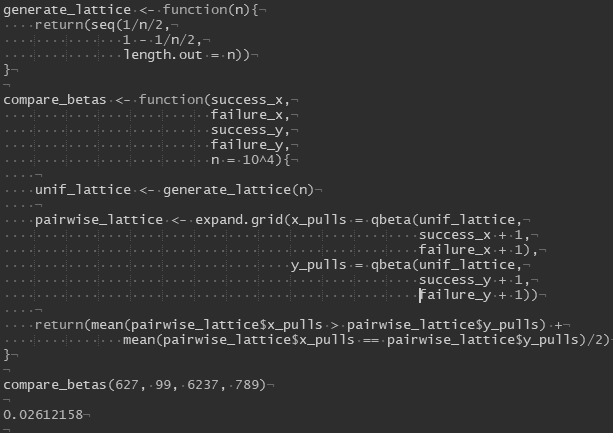
So now what? What does this do for me? I pick an n of 1,000 or 10,000 or whatever and now I can… plot the CDF of (in my case) a beta distribution in a way that looks smooth and isn’t random. Where this comes in handy at least for my purposes is when I want to know how two different random variables interact. More specifically, the likelihood that one is larger than the other.5 This is relatively straightforward as an idea if you have the RAM (and the time), but I then iterate over all pairwise combinations and compare. This gives me a very good estimate of the actual likelihood, without the variability of MC sampling or the psychic damage of convolutional integrals. Now in R I can I estimate my confidence in Steve Kerr’s “true”6 career regular season FT% being higher than Reggie Miller’s7:
About a 2.6% chance by this method.8 I’ve found this handy for A/B Test evaluation, comparing two variables with different underlying distributions, and distracting myself while other people are talking to me about something way more important.
This sounds like a brag, but it’s really condemnation of everything I’m about to write. “Two economists see a $100 bill on the ground…”
I chose uniform gaps here, treating 0 and 1 like wraparound points. There might be an argument for some moment matching here, choosing a gap that ensures the variance of the percentile lattice array is 1/12 for all n > 1 to align with the reality of the uniform distribution. As it stands, the lattice is overly disperse, which I’m choosing to call a conservative choice for estimation. I’m thinking with sufficiently large n there isn’t much of a difference.
Ok you called my bluff. I’m pretty confident this is the case, maybe you have to pick a different way of generating the lattice to make this as powerful as possible. Proofs are where I know just enough math to be dangerous but not nearly enough to be actually effective.
This is a caveat about independence.
The hypothetical “true”, as opposed to whatever we observed in reality, which is a realization of the true rate.
I was really just looking for a couple of recognizable players with similar FT% but wildly different sample sizes. The former shot 627 for 726 (86.4%, surely someone has pointed this palindrome out to him before? Also! Kerr missed exactly 99 regular season FTs. Think he knew towards the end he was close to 100?) from the line over his career, the latter 6,237 for 7,026 (88.8%) according to nba.com.
Sorry for the stray, Steve.


